为网友们分享了相关的编程文章,网友张安然根据主题投稿了本篇教程内容,涉及到二维正态分布采样、置信椭圆绘制、正态分布采样、二维正态分布采样置信椭圆绘制相关内容,已被943网友关注,下面的电子资料对本篇知识点有更加详尽的解释。
二维正态分布采样置信椭圆绘制
二维正态分布采样后,绘制置信椭圆
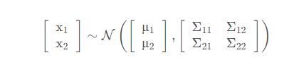
假设二维正态分布表示为:
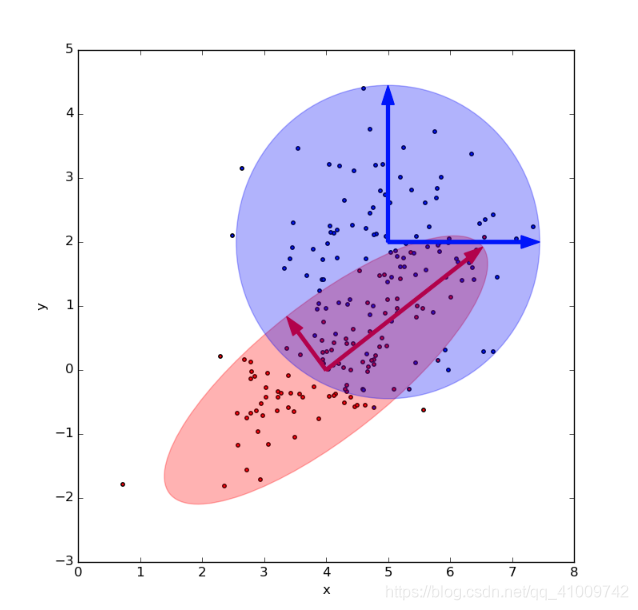
下图为两个二维高斯分布采样后的置信椭圆
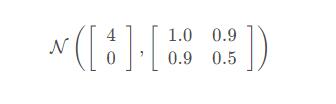
和
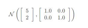
每个二维高斯分布采样100个数据点,图片为:
代码如下
#!/usr/bin/env python
# -*- coding: utf-8 -*-

import numpy as np
import matplotlib as mpl
import matplotlib.pyplot as plt

def make_ellipses(mean, cov, ax, confidence=5.991, alpha=0.3, color="blue", eigv=False, arrow_color_list=None):
    """
    多元正态分布
    mean: 均值
    cov: 协方差矩阵
    ax: 画布的Axes对象
    confidence: 置信椭圆置信率 # 置信区间, 95%: 5.991  99%: 9.21  90%: 4.605
    alpha: 椭圆透明度
    eigv: 是否画特征向量
    arrow_color_list: 箭头颜色列表
    """
    lambda_, v = np.linalg.eig(cov)    # 计算特征值lambda_和特征向量v
    # print "lambda: ", lambda_
    # print "v: ", v
    # print "v[0, 0]: ", v[0, 0]

    sqrt_lambda = np.sqrt(np.abs(lambda_))    # 存在负的特征值, 无法开方,取绝对值

    s = confidence
    width = 2 * np.sqrt(s) * sqrt_lambda[0]    # 计算椭圆的两倍长轴
    height = 2 * np.sqrt(s) * sqrt_lambda[1]   # 计算椭圆的两倍短轴
    angle = np.rad2deg(np.arccos(v[0, 0]))    # 计算椭圆的旋转角度
    ell = mpl.patches.Ellipse(xy=mean, width=width, height=height, angle=angle, color=color)    # 绘制椭圆

    ax.add_artist(ell)
    ell.set_alpha(alpha)
    # 是否画出特征向量
    if eigv:
        # print "type(v): ", type(v)
        if arrow_color_list is None:
            arrow_color_list = [color for i in range(v.shape[0])]
        for i in range(v.shape[0]):
            v_i = v[:, i]
            scale_variable = np.sqrt(s) * sqrt_lambda[i]
            # 绘制箭头
            """
            ax.arrow(x, y, dx, dy,    # (x, y)为箭头起始坐标,(dx, dy)为偏移量
                     width,    # 箭头尾部线段宽度
                     length_includes_head,    # 长度是否包含箭头
                     head_width,    # 箭头宽度
                     head_length,    # 箭头长度
                     color,    # 箭头颜色
                     )
            """
            ax.arrow(mean[0], mean[1], scale_variable*v_i[0], scale_variable * v_i[1],
                     width=0.05,
                     length_includes_head=True,
                     head_width=0.2,
                     head_length=0.3,
                     color=arrow_color_list[i])
            # ax.annotate("",
            #             xy=(mean[0] + lambda_[i] * v_i[0], mean[1] + lambda_[i] * v_i[1]),
            #             xytext=(mean[0], mean[1]),
            #             arrowprops=dict(arrowstyle="->", color=arrow_color_list[i]))


    # v, w = np.linalg.eigh(cov)
    # print "v: ", v

    # # angle = np.rad2deg(np.arccos(w))
    # u = w[0] / np.linalg.norm(w[0])
    # angle = np.arctan2(u[1], u[0])
    # angle = 180 * angle / np.pi
    # s = 5.991   # 置信区间, 95%: 5.991  99%: 9.21  90%: 4.605
    # v = 2.0 * np.sqrt(s) * np.sqrt(v)
    # ell = mpl.patches.Ellipse(xy=mean, width=v[0], height=v[1], angle=180 + angle, color="red")
    # ell.set_clip_box(ax.bbox)
    # ell.set_alpha(0.5)
    # ax.add_artist(ell)

def plot_2D_gaussian_sampling(mean, cov, ax, data_num=100, confidence=5.991, color="blue", alpha=0.3, eigv=False):
    """
    mean: 均值
    cov: 协方差矩阵
    ax: Axes对象
    confidence: 置信椭圆的置信率
    data_num: 散点采样数量
    color: 颜色
    alpha: 透明度
    eigv: 是否画特征向量的箭头
    """
    if isinstance(mean, list) and len(mean) > 2:
        print "多元正态分布,多于2维"
        mean = mean[:2]
        cov_temp = []
        for i in range(2):
            cov_temp.append(cov[i][:2])
        cov = cov_temp
    elif isinstance(mean, np.ndarray) and mean.shape[0] > 2:
        mean = mean[:2]
        cov = cov[:2, :2]
    data = np.random.multivariate_normal(mean, cov, 100)
    x, y = data.T
    plt.scatter(x, y, s=10, c=color)
    make_ellipses(mean, cov, ax, confidence=confidence, color=color, alpha=alpha, eigv=eigv)


def main():
    # plt.figure("Multivariable Gaussian Distribution")
    plt.rcParams["figure.figsize"] = (8.0, 8.0)
    fig, ax = plt.subplots()
    ax.set_xlabel("x")
    ax.set_ylabel("y")
    print "ax:", ax

    mean = [4, 0]
    cov = [[1, 0.9],
           [0.9, 0.5]]

    plot_2D_gaussian_sampling(mean=mean, cov=cov, ax=ax, eigv=True, color="r")

    mean1 = [5, 2]
    cov1 = [[1, 0],
           [0, 1]]
    plot_2D_gaussian_sampling(mean=mean1, cov=cov1, ax=ax, eigv=True)

    plt.savefig("./get_pickle_data/pic/gaussian_covariance_matrix.png")
    plt.show()


if __name__ == "__main__":
    main()
总结
以上为个人经验,希望能给大家一个参考,也希望大家多多支持码农之家。