给大家整理了相关的编程文章,网友范斯玉根据主题投稿了本篇教程内容,涉及到Python遗传算法、Python优化算法、Python遗传算法相关内容,已被715网友关注,涉猎到的知识点内容可以在下方电子书获得。
Python遗传算法
一、前言
优化算法,尤其是启发式的仿生智能算法在最近很火,它适用于解决管理学,运筹学,统计学里面的一些优化问题。比如线性规划,整数规划,动态规划,非线性约束规划,甚至是超参数搜索等等方向的问题。
但是一般的优化算法还是matlab里面用的多,Python相关代码较少。
我在参考了一些文章的代码和模块之后,决定学习scikit-opt这个模块。这个优化算法模块对新手很友好,代码简洁,上手简单。而且代码和官方文档是中国人写的,还有很多案例,学起来就没什么压力。
缺点是包装的算法种类目前还不算多,只有七种:(差分进化算法、遗传算法、粒子群算法、模拟退火算法、蚁群算法、鱼群算法、免疫优化算法)
本次带来的是数学建模里面经常使用的遗传算法的使用演示。
二、安装
首先安装模块,在cmd里面或者anaconda prompt里面输入:
pip install scikit-opt
对于当前开发人员版本:
git clone git@github.com:guofei9987/scikit-opt.git
cd scikit-opt
pip install .
三、遗传算法
3.1 自定义函数
UDF(用户定义函数)现已推出!
例如,您刚刚制定了一种新型函数。现在,你的函数是这样的:
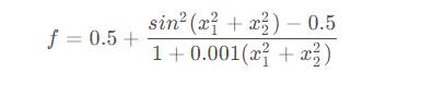
该函数有大量的局部最小值,具有很强的冲击力,在(0,0) 处的全局最小值,值为 0。
import numpy as np
def schaffer(p):
    x1, x2 = p
    x = np.square(x1) + np.square(x2)
    return 0.5 + (np.square(np.sin(x)) - 0.5) / np.square(1 + 0.001 * x)
导入和构建 ga :(遗传算法)
from sko.GA import GA
ga = GA(func=schaffer, n_dim = 2, size_pop = 100, max_iter = 800, prob_mut = 0.001, lb = [-1, -1], ub = [1, 1], precision = 1e-7)
best_x, best_y = ga.run()
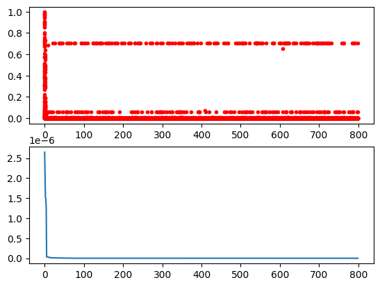
print('best_x:', best_x, '\n', 'best_y:', best_y)运行结果为:
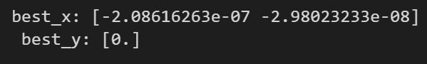
可以看到基本找到了全局最小值和对应的x 。
画出迭代次数的图:
import pandas as pd
import matplotlib.pyplot as plt
Y_history = pd.DataFrame(ga.all_history_Y)
fig, ax = plt.subplots(2, 1)
ax[0].plot(Y_history.index, Y_history.values, '.', color = 'red')
Y_history.min(axis = 1).cummin().plot(kind = 'line')
plt.show()
GA算法的参数详解:
输入参数:
| 输入参数 | 默认值 | 参数的意义 |
|---|---|---|
| func | - | 目标函数 |
| n_dim | - | 目标函数的维度 |
| size_pop | 50 | 种群规模 |
| max_iter | 200 | 最大迭代次数 |
| prob_mut | 0.001 | 变异概率 |
| lb | -1 | 每个自变量的最小值 |
| ub | 1 | 每个自变量的最大值 |
| constraint_eq | 空元组 | 等式约束 |
| constraint_ueq | 空元组 | 不等式约束 |
| precision | 1e-7 | 精确度,int / float或者它们组成的列表 |
输出参数:
GA & GA_TSP
| 输出参数 | 参数的意义 |
|---|---|
| ga.generation_best_X | 每一代的最优函数值对应的输入值 |
| ga.generation_best_Y | 每一代的最优函数值 |
| ga.all_history_FitV | 每一代的每个个体的适应度 |
| ga.all_history_Y | 每一代每个个体的函数值 |
3.2 遗传算法进行整数规划
在多维优化时,想让哪个变量限制为整数,就设定 precision 为 整数 即可。
例如,我想让我的自定义函数的某些变量限制为整数+浮点数(分别是整数,整数,浮点数),那么就设定 precision=[1, 1, 1e-7]
例子如下:
from sko.GA import GA
demo_func = lambda x: (x[0] - 1) ** 2 + (x[1] - 0.05) ** 2 + x[2] ** 2
ga = GA(func = demo_func, n_dim = 3, max_iter = 500, lb = [-1, -1, -1], ub = [5, 1, 1], precision = [1,1,1e-7])
best_x, best_y = ga.run()
print('best_x:', best_x, '\n', 'best_y:', best_y)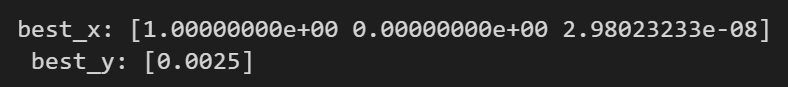
可以看到第一个、第二个变量都是整数,第三个就是浮点数了 。
3.3 遗传算法用于旅行商问题
商旅问题(TSP)就是路径规划的问题,比如有很多城市,你都要跑一遍,那么先去哪个城市再去哪个城市可以让你的总路程最小。
实际问题需要一个城市坐标数据,比如你的出发点位置为(0,0),第一个城市离位置为 ( x 1 , y 1 ) (x_1,y_1) (x1,y1),第二个为 ( x 2 , y 2 ) (x_2,y_2) (x2,y2)…这里没有实际数据,就直接随机生成了。
import numpy as np
from scipy import spatial
import matplotlib.pyplot as plt
num_points = 50
points_coordinate = np.random.rand(num_points, 2)  # generate coordinate of points
points_coordinate
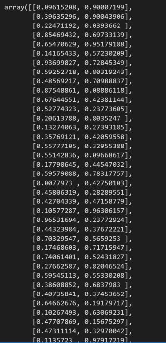
这里定义的是50个城市,每个城市的坐标都在是上图随机生成的矩阵。
然后我们把它变成类似相关系数里面的矩阵:
distance_matrix = spatial.distance.cdist(points_coordinate, points_coordinate, metric='euclidean')
distance_matrix.shape
(50, 50)
这个矩阵就能得出每个城市之间的距离,算上自己和自己的距离(0),总共有2500个数。
定义问题:
def cal_total_distance(routine):
    num_points, = routine.shape
    return sum([distance_matrix[routine[i % num_points], routine[(i + 1) % num_points]] for i in range(num_points)])
求解问题:
from sko.GA import GA_TSP
ga_tsp = GA_TSP(func = cal_total_distance, n_dim = num_points, size_pop = 50, max_iter = 500, prob_mut = 1)
best_points, best_distance = ga_tsp.run()
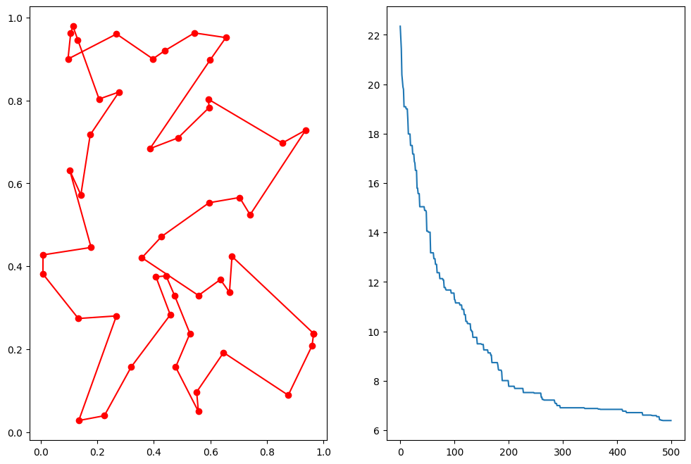
我们展示一下结果:
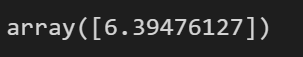
best_distance
画图查看计算出来的路径,还有迭代次数和y的关系:
fig, ax = plt.subplots(1, 2,figsize = (12, 8))
best_points_ = np.concatenate([best_points, [best_points[0]]])
best_points_coordinate = points_coordinate[best_points_, :]
ax[0].plot(best_points_coordinate[:, 0], best_points_coordinate[:, 1], 'o-r')
ax[1].plot(ga_tsp.generation_best_Y)
plt.show()
3.4 使用遗传算法进行曲线拟合
构建数据集:
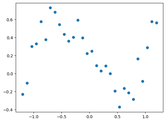
import numpy as np
import matplotlib.pyplot as plt
from sko.GA import GA
x_true = np.linspace(-1.2, 1.2, 30)
y_true = x_true ** 3 - x_true + 0.4 * np.random.rand(30)
plt.plot(x_true, y_true, 'o')
构建的数据是 y = x 3 − x + 0.4 y=x^3-x+0.4 y=x3−x+0.4,然后加上了随机扰动项。如图:
定义需要拟合的函数(三次函数),然后将残差作为目标函数去求解:
def f_fun(x, a, b, c, d):
    return a * x ** 3 + b * x ** 2 + c * x + d   #三次函数

def obj_fun(p):
    a, b, c, d = p
    residuals = np.square(f_fun(x_true, a, b, c, d) - y_true).sum()
    return residuals
求解:
ga = GA(func = obj_fun, n_dim = 4, size_pop = 100, max_iter = 500, lb = [-2] * 4, ub = [2] * 4)
best_params, residuals = ga.run()
print('best_x:', best_params, '\n', 'best_y:', residuals)
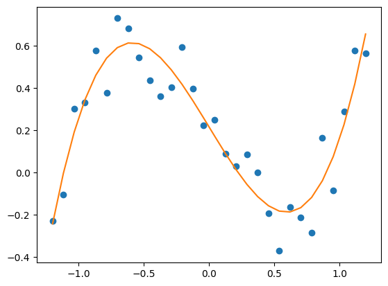
可以看到拟合出来的方程为 y = 0.9656 x 3 − 0.0065 x 2 − 1.0162 x + 0.2162 y=0.9656x^{3}-0.0065x^{2}-1.0162x+0.2162 y=0.9656x3−0.0065x2−1.0162x+0.2162
画出拟合线:
y_predict = f_fun(x_true, *best_params)
fig, ax = plt.subplots()
ax.plot(x_true, y_true, 'o')
ax.plot(x_true, y_predict, '-')
plt.show()
到此这篇关于Python优化算法—遗传算法的文章就介绍到这了,更多相关Python遗传算法内容请搜索码农之家以前的文章或继续浏览下面的相关文章希望大家以后多多支持码农之家!